student_id learnerName .pred_yes dropout
1 1 glm_predSet_bm 0.19666440 0
8000 1 glm_predSet_ms 0.09658994 0
15999 1 lasso_predSet_ms 0.08760455 0
23998 1 random_forest_predSet_ms 0.17969438 0Learner training & validation with code templates

02_Learner_Training_and_Validation
After making all specifications for your PA proof-of-concept in 01_Learner_Specification.Rmd, all the learners you defined are trained in 02_Learner_Training_and_Validation.Rmd. This training happens in the code chunk replicated below. The user does not need to enter or edit any code within the chunk. Specifications that were entered in 01_Learner_Specification.Rmd are loaded in the chunk that precedes this one and are passed into the train_learners() function.
# running model results all learners in learnerSpec (all specified in 01_Learner_Specification.Rmd)
learnersResults <- train_learners(
  learnerSpec = learnerSpec,
  recipes = recipes,
  mainRecipes = mainRecipes
)

 # this returns cross-validated means and SE for AUC-PR and AUC-ROC
modelResults <- learnersResults$modelResults
 # this is predicted probabilities, from when obs are in validation set
predProbs    <- learnersResults$predProbs
As commented in the above chunk, the code returns information about a couple of performance metrics abbreviated as AUC-PR and AUC-ROC. AUC-PR is the area under the curve (AUC) for a precision recall (PR) curve. AUC-ROC is the area under the curve (AUC) for a receiver operating characteristic (ROC) curve. We will return to explanations of these in a bit.
First, let’s focus on the other information that is returned in the above code chunk - the predicted probabilities. For each observation (unit or row) in our dataset used for training or validation, each learner produces a predicted probability of the outcome. The code returns these predicted probabilities for each observation for each learner.
For example, imagine we are predicting whether a student will drop out of high school. Then, for each student, we get the following information, displayed for just one student.
The numbers to the left (1, 8000, 15999, 23998) are the row numbers in the data.frame predProbs that correspond to the student with student_id = ‘1’. By examining the entries for learnerName, we can see that we conducted training for four different learners. These four different learners were combinations of two predictor sets (“bm” and “ms”) and three modeling approaches (“glm”, “lasso” and “random_forest”). Note that the predSet suffix of ’_bm’ signifies the “benchmark” predictor set. The suffix of ’_ms’ was chosen by the user for a second predictor set; it is not following any particular convention. The column .pred_yes tells us the probability that the outcome is equal to ‘1’. (While not displayed, predProbs also contains pred_no, the probability that the outcome is equal to ‘0’.) Finally, we also see the actual, observed outcome (dropout) for this student. The predProbs dataframe also includes all the other measures in the training/validation data; they are just not displayed here.
The predicted probabilities listed for .pred_yes were estimated through the \(v\)-fold cross-validation procedure. Recall from the earlier section on cross-validation, that each observation takes a turn in a validation fold. After a learner was trained on the \(v-1\) other folds, the resulting model was applied to the validation fold, producing a predicted probability for each observation in the validation fold.
Summarizing the predicted probabilities
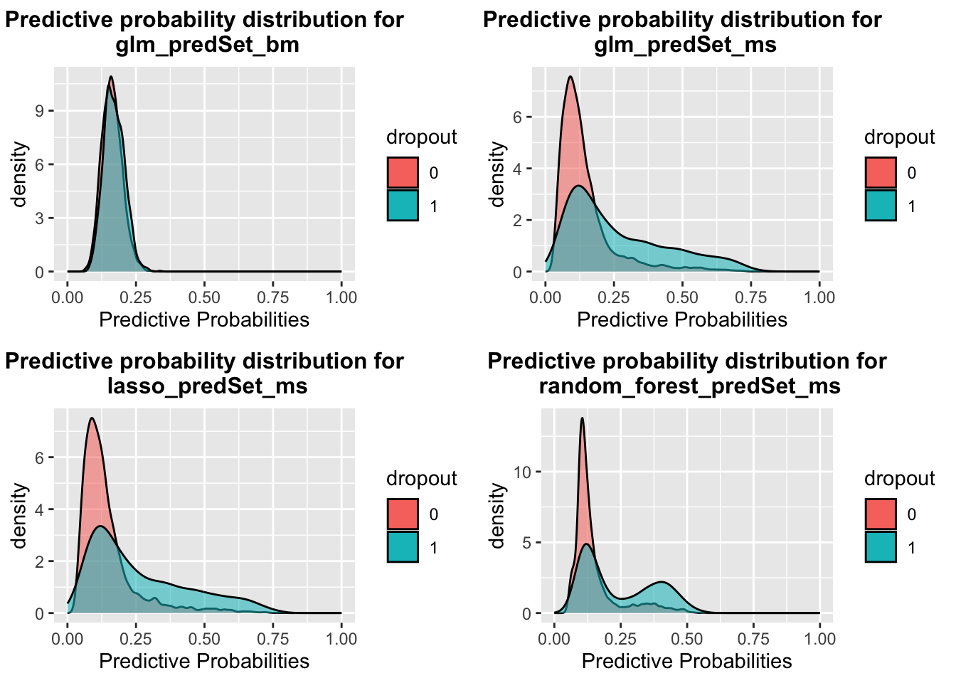
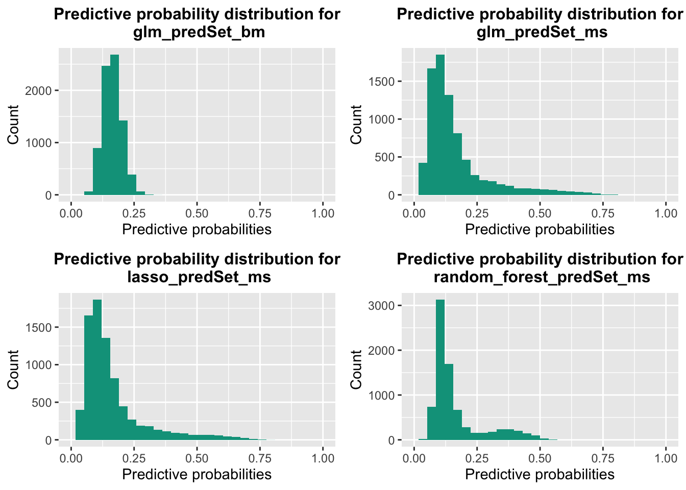
A helpful first step for understanding the validation results is to examine the distributions of the predicted probabilities. The following set of plots shows the distribution for each learner. The code chunk named “plotpredProbs” in 02_Learner_Training_and_Validation will create these plots for you.
As expected, because most students do not drop out, the predicted probabilities tend to cluster around low values. Also, note that some learners produce greater variability than others.
Next, the notebook plots overlapping distributions of predicted probabilities for when the observed outcome = ‘1’ and when the observed outcome = ‘0’. This plot illustrates how well each learner is able to separate out the predicted probabilities for the different classifications.