Threshold-invariant metrics
For some performance metrics, we do not need to specify a threshold. Here we summarize two “threshold-invariant” metrics: the AUC-ROC and AUC-PR. Remember that this code chunk from 02_Training_and_Validation.Rmd (repeated below) also returns these metrics. For these metrics, each is computed for each validation fold during the \(v\)-fold cross-validation procedure. Then the metrics are averaged across all \(v\) validation folds.
# running model results all learners in learnerSpec (all specified in 01_Learner_Specification.Rmd)
learnersResults <- train_learners(
  learnerSpec = learnerSpec,
  recipes = recipes,
  mainRecipes = mainRecipes
)

 # this returns cross-validated means and SE for AUC-PR and AUC-ROC
modelResults <- learnersResults$modelResults
 # this is predicted probabilities, from when obs are in validation set
predProbs    <- learnersResults$predProbs
AUC-ROC
AUC-ROC is the area under the curve (AUC) for a receiver operating characteristic (ROC) curve. The higher the value, the better the model is at making predictions.
An ROC curve plots FPR (1-specificity) on the \(x\)-axis against the TPR (sensitivity/recall) on the \(y\)-axis, as the threshold changes. The first point in the bottom left corner of the ROC curve corresponds to the TPR and FPR at a threshold of 1. Next, imagine we change the threshold to 0.95. Then all units with a predicted value above 0.95 will be classified as ‘1’, and all units with a predicted value below 0.95 will be classified as ‘0’. At this threshold, most of the units we classify as ‘1’ will be true observed positives, so we expect a high true positive rate and a low false positive rate. As we decrease the threshold, we will classify more and more units as ‘1’, which increases the false positive rate (numerator increases) and decreases the true positive rate (denominator increases). A good model has a high true positive rate and a low false positive rate, so points farther to the left and farther up are markers of a good model.
We usually compare a model’s curve to a line that goes straight up the diagonal from 0 to 1. This line corresponds to the performance of a random classifier. A random classifier picks the class of each unit using a random coin flip, without any information about the unit. Ideally, a trained model informed by the patterns in the data performs much better than a random classifier.
The AUC-ROC measures how well predictions are ranked, rather than their absolute values. Therefore, the measure is helpful when you want to target a service, marketing campaign, intervention, etc. to those most or least likely to have a positive outcome.
In the case of imbalanced data, when one of the categories is very rare, ROC curves can give misleading results and be overly optimistic of model performance. As a rule of thumb, if your data has 10% or less of units in one category, you may have imbalanced data. In this case, AUC of precision recall curve, discussed next, may be a better metric. For more information about imbalanced data, see our short explainer attached in the reference folder on the subject, and why ROC curves may not perform well in that setting.
This code chunk in 02_Learner_Training_and_Validation.Rmd plots ROC curves for each specified learner.
# running model results all learners in learnerSpec (all specified in 01_Learner_Specification.Rmd)
learnersResults <- train_learners(
  learnerSpec = learnerSpec,
  recipes = recipes,
  mainRecipes = mainRecipes
)

 # this returns cross-validated means and SE for AUC-PR and AUC-ROC
modelResults <- learnersResults$modelResults
 # this is predicted probabilities, from when obs are in validation set
predProbs <- learnersResults$predProbs 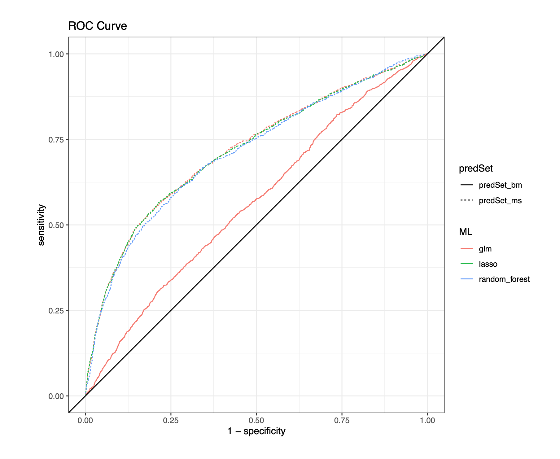
AUC-PR
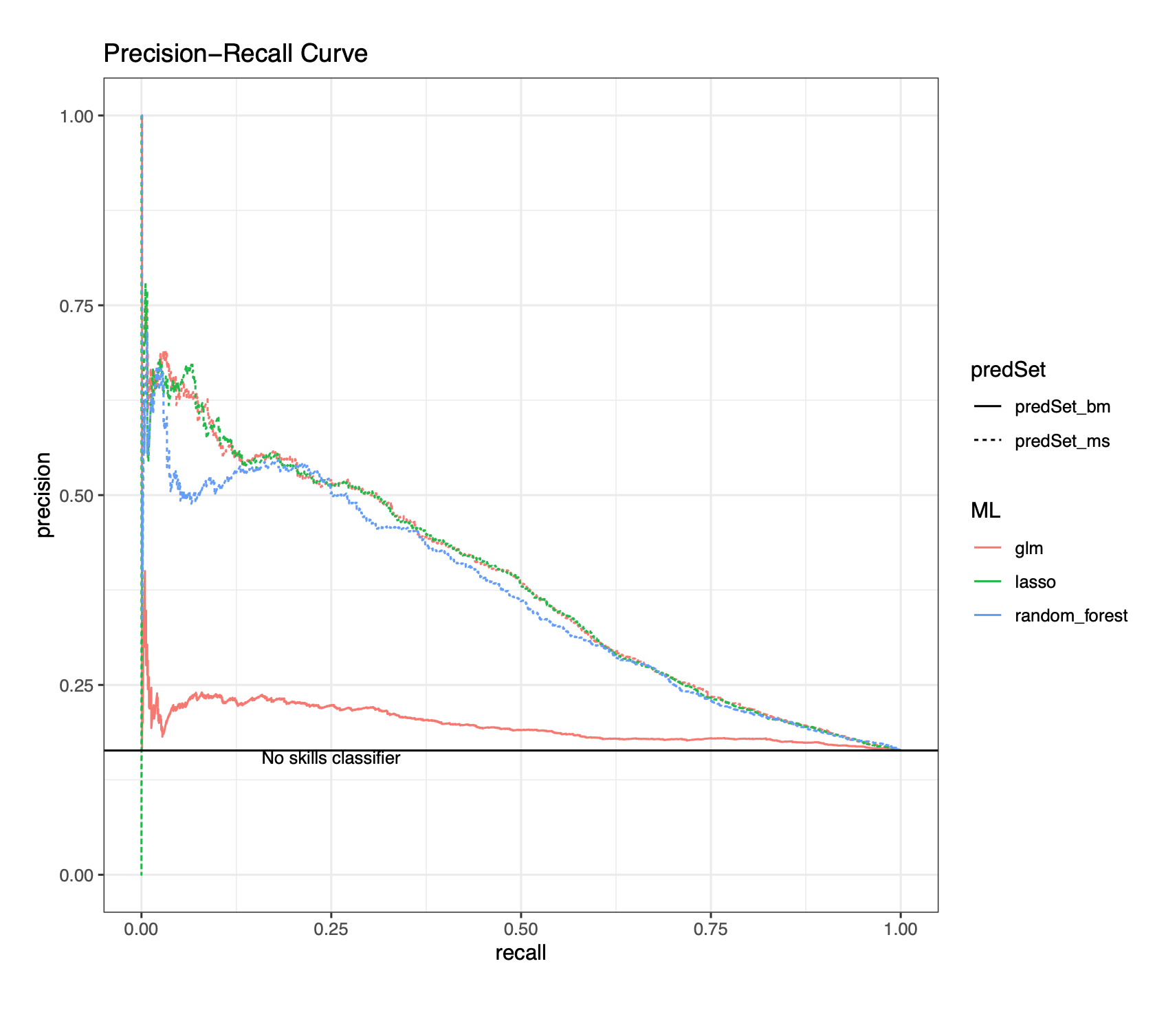
AUC-PR is area under the curve (AUC) for a precision recall (PR) curve. For the PR curve, the true positive rate (sensitivity/recall) is on the \(x\)-axis and the positive predicted value (precision) is on the \(y\)-axis. Like in AUC ROC as well, the precision and recall are plotted as the threshold changes.
AUC-PR is a valuable metric when there is class imbalance, the positive class is of particular interest, and both types of classification errors (false positives and false negatives) carry significant consequences. Because AUC-PR does not account for true negatives, it is often preferred over AUC-ROC when outcome classes are imbalanced. With a rare outcome, the FPR tends to remain low due to a large number of observed negatives. Recall that FPR = FP/(TN + FP). A larger number of observed negative values within the imbalanced data would imply a large denominator (because TN would be large) and hence, we would see a low false positive rate even as the number of false positives increases. Thus, AUC-ROC can be a less informative and at times overly optimistic metric for imbalanced data.
AUC PR, on the other hand, is a trade-off between precision (TP/(TP + FP)) and recall/sensitivity (TP/(TP + FN)). Precision is solely based on predicted positive values (TP and FP) and is unaffected if there is a large number of observed negatives. If there are few false positives, then there will be both a low false positive rate (smaller numerator for FPR) and high precision (smaller denominator for precision). If there are few false negatives, then there will be both a low false negative rate (smaller numerator for FNR) and a high recall (smaller denominator for recall). Therefore, a high AUC PR score is good because it implies low false positive and false negative rates (just like a high AUC ROC score).
This code chunk in 02_Learner_Training_and_Validation.Rmd plots PR curves for each specified learner.
# running model results all learners in learnerSpec (all specified in 01_Learner_Specification.Rmd)
learnersResults <- train_learners(
  learnerSpec = learnerSpec,
  recipes = recipes,
  mainRecipes = mainRecipes
)

 # this returns cross-validated means and SE for AUC-PR and AUC-ROC
modelResults <- learnersResults$modelResults
 # this is predicted probabilities, from when obs are in validation set
predProbs    <- learnersResults$predProbs